10 Tips and Tricks to Up Your Excel and Google Sheets Game

Working and knowing how to use Excel and Google sheets properly is a skill and talent in itself. A lot of us spend a large chunk of our time using Excel and Google sheets without ever truly knowing the many features or hacks that are created to make our work easier. In this blog, you’re going to learn shortcuts for excel and Google sheets tips and tricks that will make your life much easier.  

Source: Excel Easy

Excel and sheets are essential in our professional fields, and it is important to know how to use excel for work. Here are just some of the many things you can do working on excel:

One of the most popular sorts of documents you may produce using Excel is a balance sheet. It allows you to gain a comprehensive picture of a company's financial position. You can also quickly make a monthly calendar in a spreadsheet to keep track of events or other date-sensitive information. Excel is a powerful budgeting tool, it may be used to set and track marketing budgets as well as spend. If you don't use a marketing solution like Marketing Hub, you might require a dashboard to keep track of all of your reports. Excel is a fantastic programme for creating marketing reports. It can also make editorial calendars which makes tracking your content development efforts over unique time periods a breeze. Excel is a wonderful tool for creating all kinds of calculators, including one for tracking leads and traffic, thanks to its powerful computational capabilities. Here are some of the most useful Google Sheets tips and tricks, as well as how to get better at Excel:

1. Remove any leading or trailing spaces: This tip will offer you a cleaner version of the cell's value in Excel or Google Sheets. Don't forget about the Google Sheets function TRIM if you notice some excess spaces before or after data in your spreadsheet (whether you're looking at numbers or text). You can enter it in for whatever cell you want (for example, =TRIM(A1)) and it will work.

2. Freeze Rows: Simply place your cursor on the bottom of the first cell right above "1" and to the left of "A" in any spreadsheet's upper-left corner. When the hand symbol appears, click it and drag down for as many rows as you wish to freeze before letting go. No matter how far you scroll down, the rows you select will always be in place and displayed at the top of your spreadsheet.

3. Pull data from publicly available web pages: Working on excel, you can also get data from any publicly available web page with a correctly prepared table. The key is to use the ImportHTML command with any URL and a number specifying which table on the page you want to import ("1" for the first table, "2" for the second, and so on): 

=IMPORTHTML("https://en.wikipedia.org/wiki/Type_of_data","table",1)

4. Make good pie charts: Another set of Excel tips and tricks, try clicking twice on one specific piece of the pie chart and then looking for the Distance from centre option in the control panel on the right side of the screen the next time you create a pie chart in a spreadsheet—by highlighting cells and then clicking the Insert menu followed by Chart (and then clicking Chart type to select a pie chart option if one doesn't come up by default). Increase its value to at least 25% to make that section of the chart stand out for emphasis.

5. Create a functional checklist: Select a group of blank cells, then choose Checkbox from the Insert menu. You can then move your to-do items to the next column and enjoy the satisfaction of crossing things off your list as you finish them.

6. Sheets can be linked to other services: Since sheets live in a web browser and are connected by default, it makes sense to connect it to other web-based services. You can grab data from other sources like Twitter, Instagram, and more thanks to connectivity services like IFTTT and Zapier. Instead of downloading data from those services and reformatting it for Sheets, you can use these services to sit in the middle and automatically share data between the services.

7. Make a chart in a single cell: Using Sheets' handy Sparkline function, make a little chart in a single cell. Simply type =Sparkline, followed by the cells you want to include, the term "charttype," and the chart type you want to create—such as line, bar, or column—in this format:

=SPARKLINE(E12:E23,{"charttype","column"})

8. Collect data over the web using a survey-style form:  You can make a form by going to Sheets Insert menu and selecting Form, then utilising the webpage that appears to create any set of questions and criteria you desire. When your form is finished, click the Send button in the upper-right corner of the page to email it, embed it in a web page, or obtain a manual link to share it however you like. As responses come in, they'll appear in your spreadsheet as separate rows in your spreadsheet.

9. Create QR codes: Sheets can build a QR code that, when scanned, will bring up any URLs you want, thanks to the support of an external provider. Put your URL in a cell (with http:// or https:// in front of it), then use the following function to replace "B4" with your own cell number:

=image("https://image-charts.com/chart?chs=150x150&cht=qr&choe=UTF-8&chl="&ENCODEURL(B4))

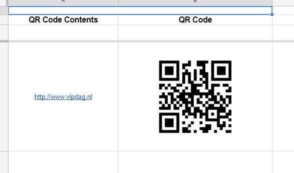
Source: Stack Overflow

10. Get real time historical stock prices along with all sorts of other market-related data: For your stock-knowledge needs, Sheets has Google Finance built right in. For every publicly traded firm, the system can provide you with real-time or historical stock prices, as well as a variety of other market-related data. Simply use the GoogleFinance function, followed by the data you want to see, and the variables and formats provided here.

Here are some shortcuts for sheets and excel keyboard shortcuts that can also improve your Excel and Sheets game:

• AVERAGE: The AVERAGE function takes the values of a group of cells and averages them out. The AVERAGE function has the same syntax as the SUM function: (Cell1:Cell2). =AVERAGE is a good example (C5:C30).
• IF: You can use the IF function to return values depending on a logical test. The following is the syntax: If (logical test, value if true, [value if false]) is true, then =IF(A2>B2,"Over Budget","OK"), for example.
• VLOOKUP: The VLOOKUP function allows you to search for anything in the rows of your sheet. VLOOKUP(lookup value, table array, column number, Approximate match (TRUE) or Exact match (FALSE)) is the syntax. =VLOOKUP([@Attorney],tbl Attorneys,4,FALSE), for example.
• INDEX: INDEX returns a value from a range. Here's how to write it: INDEX(array, row num, [column num]) is a function that returns the number of rows and columns in the array.
• MATCH: The MATCH function searches a range of cells for a specific object and returns its location. It can work in conjunction with the INDEX function. MATCH(lookup value, lookup array, [match type]) is the syntax.
• COUNTIF: The COUNTIF function calculates the number of cells that fulfil a set of conditions or have a specific value. COUNTIF is the formula (range, criteria). for example, =COUNTIF=, (A2:A5,"America").